2022. 3. 7. 15:46ㆍ책/누구나 자료 구조와 알고리즘
친구 관계를 데이터로 조직한다고 해보자. 어떤 방식으로 만들겠는가? 단순하게는 배열로 저장해볼 수 있겠다.
친구관계 = [ ["A","B"], ["B","C"], ["A","C"], ["B","D"], ["E","F"], ... ]
불행히도 A의 친구가 누구인지 확인도 어렵고, 컴퓨터는 확인을 위해 일일이 배열을 뒤져봐야 하므로 O(N)이 걸리는 매우 느린 방법이다. 이럴 때 그래프라는 자료 구조를 사용하면 O(1) 시간 만에 찾아낼 수 있다.
1. 그래프
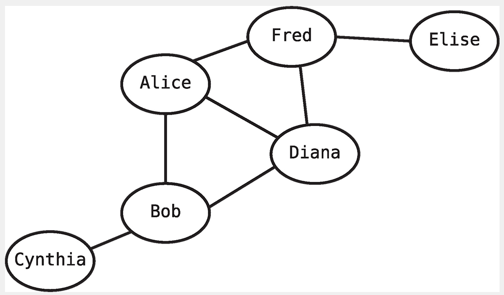
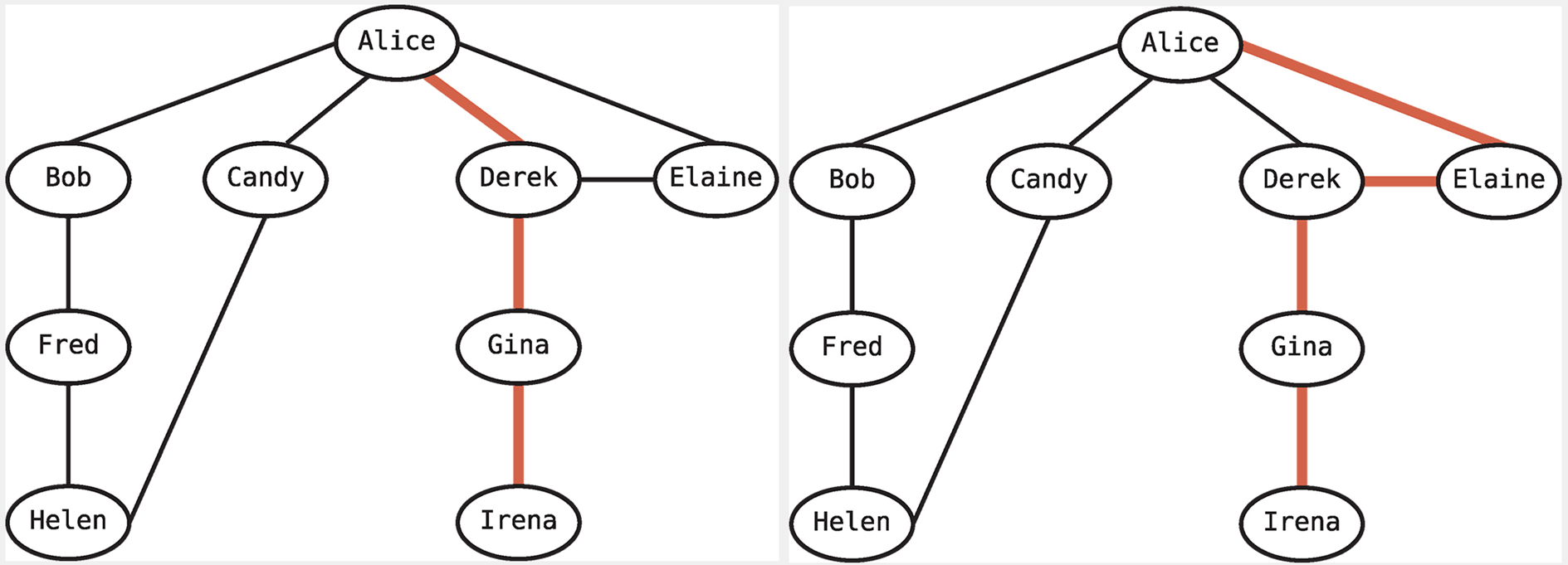
관계에 특화된 자료 구조로서 데이터가 연결된 모습을 쉽게 이해시켜 준다. 아래 그림처럼 사람을 노드로, 관계를 선으로 표현한다. 진짜로
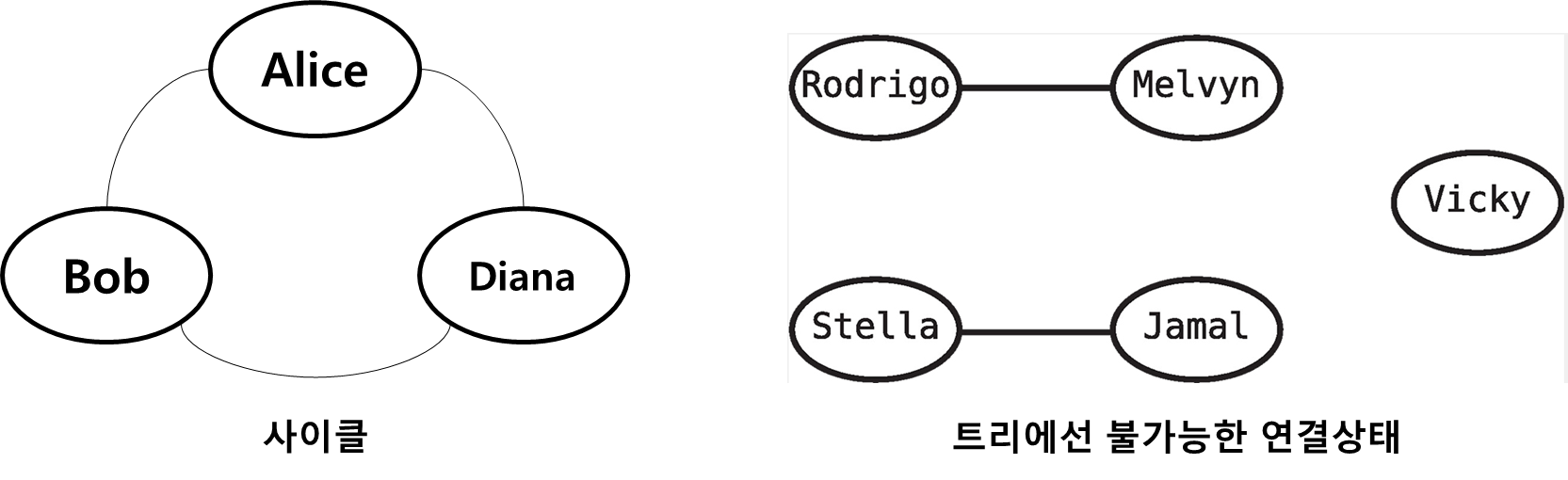
1.1 그래프 vs 트리
사실 트리도 노드들이 서로 연결돼있는 자료구조였다. 그럼 트리도 그래프 아닌가? 맞다. 사실 트리도 그래프의 한 종류다. 즉, 모든 트리는 그래프이지만, 그래프가 모두 트리인 것은 아니다. 구체적으로는
- 트리에는 사이클이 있을 수 없으며, 모든 노드가 서로 연결되어야 한다
- 트리의 모든 노드는 다른 노드와 연결된다
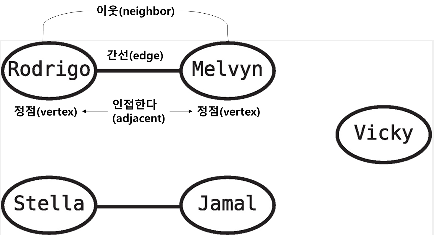
1.2 그래프 용어
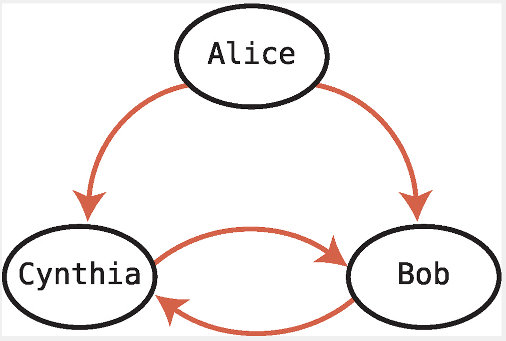
2. 방향 그래프(directed graph)
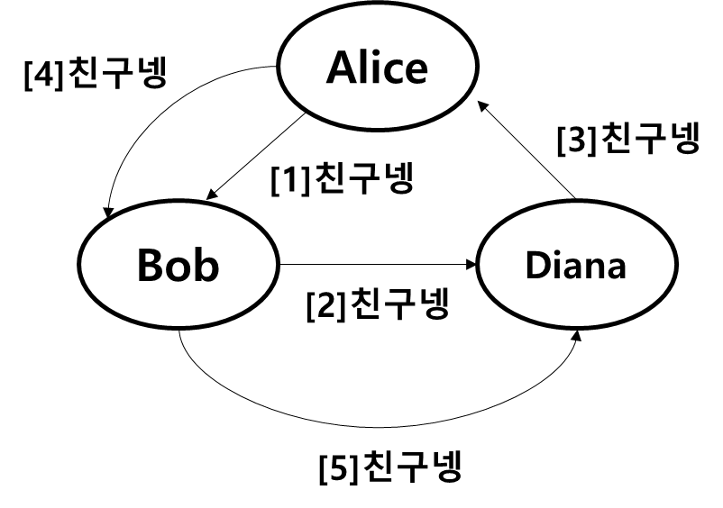
인스타에서 앨리스가 밥을 팔로우하지만, 밥은 앨리스를 팔로우하지 않을 수도 있다. 이처럼 관계의 방향성이 존재하는 그래프를 방향 그래프라고 부른다.
3. 그래프 구현
위 그림을 그래프로 구현하면 다음과 같다. 방향 그래프버전과 무방향 그래프 버전을 모두 표기해놨음
class Vertex {
    #value;
    #adjacentVertices = [];

    constructor(value) {
        this.#value = value;
    }

    get value() {
      return this.#value
    };

    set value(value) {
      this.#value = value
    };

    get adjacentVertices() {
      return this.#adjacentVertices
    };

    set adjacentVertices(adjacentVertices) {
      this.#adjacentVertices = adjacentVertices
    };

    // 방향그래프 ver
    addAdjacentVertex(vertex) {
      this.#adjacentVertices.push(vertex)
    }

    // 무방향그래프 ver
    addAdjacentVertex(vertex) {
        if (this.#adjacentVertices.include(vertex)) return;
        this.#adjacentVertices.push(vertex);
        vertex.addAdjacentVertex(this)
    }
}

const alice = new Vertex('alice');
const bob = new Vertex('bob');
const cynthia = new Vertex('cynthia');

alice.addAdjacentVertex('bob');
alice.addAdjacentVertex('cynthia');
bob.addAdjacentVertex('cynthia');
cynthia.addAdjacentVertex('bob');
단순하게 설명하기 위해 앞으로는 연결된 그래프만 다뤄보도록 하자. 연결 그래프는 Vertex 클래스 하나로 앞으로 나올 모든 알고리즘을 다룰 수 있다.
4. 그래프 탐색
먼저 그래프 용어의 '탐색' 이란 말은 두 가지로 쓰일 수 있다.
- 그래프내 한 정점을 찾는다
- 그래프 내 한 정점에 접근 가능할 떄, 그 정점과 연결된 또 다른 정점을 찾는다.
두번째 탐색이 무슨소리냐면 A 정점에 접근할 수 있을 때, B 정점을 탐색한다 = A → B의 경로를 찾는다 라는 뜻이다.
그래프 탐색에는 깊이 우선 탐색과 너비 우선 탐색 두 방식이 널리 쓰이는데, 뒤에서 알아보자.
5. 깊이 우선 탐색
이진 트리 순회 알고리즘과 매우 유사하다. 다만, 그래프는 사이클이 존재할 수 있으므로 영원히 순회하는 경우가 발생할 수 있으니 주의해야 한다.
이를 해결하는 한 방법으로 방문했던 정점을 해시 테이블에 불리언으로 저장해두는 방법이 있다.
[1] 그래프 내 임의의 정점에서 시작한다
[2] 현재 정점을 해시 테이블에 추가해 방문표시를 남긴다
[3] 현재 정점의 인접 정점을 순회한다
[4] 방문했던 인접 정점이면 무시한다
[5] 방문하지 않았던 인접 정점이면 해당 정점에 대해 재귀적으로 깊이 우선 탐색을 수행한다
5.1 깊이 우선 순회
먼저 깊이 우선 순회를 구현해보자. 즉, A라는 정점에서 시작해 인접한 모든 정점을 순회하는 코드다
dfsTraverse(vertex, visitedVertices={}) {
        // 정점을 해시 테이블에 추가해 방문했다고 표시한다.
        visitedVertices[vertex.value] = true;

        // 정점의 값을 출력해 제대로 순회하는지 확인한다.
        console.log(vertex.value);

        // 현재 정점의 인접 정점을 순회한다.
        vertex.adjacentVertices.forEach((adjacentVertex) => {
          // 이미 방문했던 인접 정점은 무시한다.
          if (visitedVertices[adjacentVertex.value]) return;

          // 인접 정점에 대해 메서드를 재귀적으로 호출한다.
          this.dfsTraverse(adjacentVertex, visitedVertices)
        })
    }
5.2 깊이 우선 탐색
앞선 코드는 모든 정점을 순회하는 코드였고, 이번엔 실제로 어떤 정점을 찾는 코드를 구현해보자.
dfs(vertex, searchValue, visitedVertices={}) {
        // 찾고 있던 정점이면 원래의 vertex을 반환한다.
        if (vertex.value == searchValue) return vertex;
        visitedVertices[vertex.value] = true;

        let resultVertex = null;

        vertex.adjacentVertices.forEach((adjacentVertex) => {
          if (visitedVertices[adjacentVertex.value]) return;

          // 인접 정점이 찾고 있던 정점이면
          // 그 인접 정점을 반환한다.
          if (adjacentVertex.value == searchValue) {
              resultVertex = adjacentVertex;
            }

          // 인접 정점에 메서드를 재귀적으로 호출해
          // 찾고 있던 정점을 계속 찾는다.
          let vertexWereSearchingFor = this.dfs(
            adjacentVertex,
            searchValue,
            visitedVertices
          );

          // 위 재귀에서 올바른 정점을 찾았다면
          // 그 정점을 반환한다.
          if (vertexWereSearchingFor) {
              resultVertex = vertexWereSearchingFor;
          }
        });

        // 찾고 있던 정점을 찾지 못했으면 null이 반환된다
        return resultVertex
      }
6. 너비 우선 탐색(BFS; Breadth-First Search)
깊이 우선 탐색과 달리 재귀를 쓰지 않고 큐를 쓰는 방법. 너비 순회 알고리즘은 다음과 같다.
[1] 그래프 내 아무 정점에서나 시작한다 (이 정점을 '시작 정점'이라고 부른다)
[2] 시작 정점을 해시 테이블에 추가해 방문 표시를 남긴다
[3] 시작 정점을 큐에 추가한다
[4] 큐가 빌 때까지 실행하는 루프를 시작한다
[5] 루프 안에서 큐의 첫 번째 정점을 삭제한다 (이 정점을 '현재 정점'이라고 부른다)
[6] 현재 정점의 인접 정점을 순회한다
[7] 이미 방문한 인접 정점이면 무시한다
[8] 아직 방문하지 않은 인접 정점이면 해시 테이블에 추가해 방문 표시를 남긴 후 큐에 추가한다
[9] 큐가 빌 때까지 루프를 반복한다
6.1 너비 우선 순회
bfs_traverse(startingVertex) {
        const queue = new Queue();
        const visitedVertices = {};
        visitedVertices[startingVertex.value] = true;
        queue.enqueue(startingVertex);

        while (queue.read()) {
          const currentVertex = queue.dequeue();

          console.log(currentVertex.value);
          currentVertex.adjacentVertices.forEach(adjacentVertex => {
            if (!visitedVertices[adjacentVertex.value]) {
              visitedVertices[adjacentVertex.value] = true;
              queue.enqueue(adjacentVertex);
            }
          })
        }
      }


class Queue {
  #data = [];

  enqueue(element) {
    this.#data.push(element);
  }

  dequeue() {
    return this.#data.shift();
  }

  read() {
    return this.#data[0];
  }
}
6.2 깊이 우선 vs 너비 우선
너비 우선은 시작 정점의 인접한 곳부터 훑어나가며 점차 시작 정점과 멀어진다. 반대로 깊이 우선은 탐색과 동시에 시작 정점과 최대한 멀리 떨어지려고 한다. 그럼 어떤 방법이 더 나은걸까? 당연히 상황에 따라 다르다. A라는 사람의 친구들만 찾는다고 하면 너비우선이 나을 것이다.
7. 그래프 탐색 효율성 ( O(V+E) )
그래프 탐색의 시간 복잡도를 케이스별로 분석해보자.
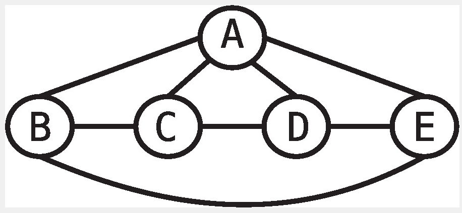
먼저 각 정점을 방문하니 기본으로 5단계가 소요된다. 그리고 간선을 오가는 단계들이 추가되는데
A : 이웃 4개를 순회하는 4단계
B : 이웃 3개를 순회하는 3단계
C : 이웃 3개를 순회하는 3단계
D : 이웃 3개를 순회하는 3단계
E : 이웃 3개를 순회하는 3단계
총 21단계가 걸린다
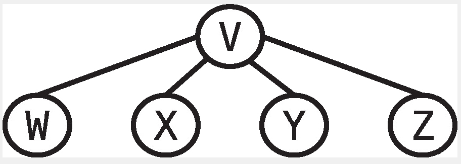
옆의 그림의 경우에도 총 13단계가 걸린다
V : 이웃 4개를 순회하는 4단계
W : 이웃 1개를 순회하는 1단계
X : 이웃 1개를 순회하는 1단계
Y : 이웃 1개를 순회하는 1단계
Z : 이웃 1개를 순회하는 1단계
즉, 정점의 수 + 2*간선의 수 (V + 2E)가 걸린다. 그리고 이를 빅 오 표기법으로 하면 O(V+E)가 걸린다. 보면 알겠지만 적절한 탐색 방법으로 간선을 오가는 단계를 줄이는게 핵심이다.
8. 가중 그래프
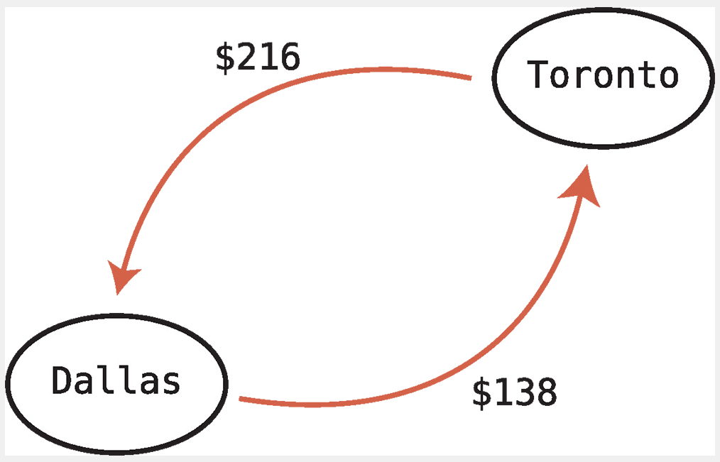
옆의 그래프처럼 두 도시를 연결하는 항공편이 있으면서 각 방향마다 항공권 가격이 다른 방향 그래프를 가중 그래프로 표현할 수 있다
- 토론토 → 댈러스 $216
- 댈러스 → 토론토 $138
가중 그래프의 이점은 최단 경로 문제를 풀기 좋다는 건데, ㄱㅈ같은 NCS에서 나오는 그 최단 경로 문제가 맞다. 여하튼 가중 그래프를 코드로 구현하면 아래와 같다
class WGraphVertex {
    #value;
    #adjacent_vertices = {};

    constructor(value) {
      this.#value = value;
    }

    get value() {
      return this.#value;
    }

    set value(element) {
      this.#value = element;
    }

    get adjacentVertices() {
      return this.#adjacent_vertices;
    }

    addAdjacentVertex(vertex, weight) {
      this.#adjacent_vertices[vertex] = weight;
    }
}

const dallas = new WGraphVertex('Dallas');
const toronto = new WGraphVertex('Toronto');
dallas.addAdjacentVertex(toronto, 138);
toronto.addAdjacentVertex(dallas, 216);
9. 데이크스트라의 알고리즘
최단 경로 문제를 푸는 알고리즘중 하나인데, 1959년 에드거 데이크스트라가 알아낸 알고리즘이라 데이크스트라 알고리즘이라고 부른다. 이 알고리즘의 최대 이점은 어디가 됐든 A → B로 가는 최단 경로를 찾아준다는 것인데, 사실 모든 도시에서 이동간 비용을 수집하기 때문에 가능하다. 아무튼 이 책에서 가장 어려운 부분이므로 잘 읽어보길 바란다.
9.1 데이크스트라 알고리즘 코드 구현
JS로 구현하기 위해 그동안 쓴 적 없던 Map 자료구조를 끼얹었고, Array의 prototype에 함수를 하나 추가했다.
class City {
#name;
#routes;
constructor(name) {
this.#name = name;
this.#routes = new Map();
}
get name() {
return this.#name;
}
set name(value) {
this.#name = value;
}
get routes() {
return this.#routes;
}
addRoute(city, price) {
this.#routes.set(city, price);
}
}
function dijkstraPath(startingCity, finalCity) {
const cheapestTable = {};
const cheapestPreviosStopoverCityTable = {};
const unvisitedCities = [];
const visitedCities = {};
cheapestTable[startingCity.name] = 0;
let currentCity = startingCity;
while(currentCity) {
visitedCities[currentCity.name] = true;
unvisitedCities.remove(currentCity);
for (const [adjacentCity, price] of currentCity.routes) {
if (!visitedCities[adjacentCity.name]) {
unvisitedCities.push(adjacentCity);
}
const priceThroughCurrentCity = cheapestTable[currentCity.name] + price;
if (!cheapestTable[adjacentCity.name] || priceThroughCurrentCity < cheapestTable[adjacentCity.name]) {
cheapestTable[adjacentCity.name] = priceThroughCurrentCity;
cheapestPreviosStopoverCityTable[adjacentCity.name] = currentCity.name;
}
}
const nextCityPriceList = [];
for (const { name } of unvisitedCities) {
nextCityPriceList.push(cheapestTable[name]);
}
const lowestCityIndex = nextCityPriceList.indexOf(Math.min(...nextCityPriceList));
currentCity = unvisitedCities[lowestCityIndex];
}
const shortestPath = [];
let currentCityName = finalCity.name;
while(currentCityName !== startingCity.name) {
shortestPath.push(currentCityName);
currentCityName = cheapestPreviosStopoverCityTable[currentCityName];
}
shortestPath.push(startingCity.name);
return shortestPath.reverse();
}
Array.prototype.remove = function(value) {
if (this.indexOf(value) !== -1) {
this.splice(this.indexOf(value),1);
}
};
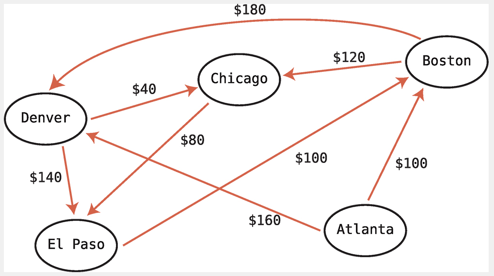
const atlanta = new City("Atlanta");
const boston = new City("Boston");
const chicago = new City("Chicago");
const denver = new City("Denver");
const elpaso = new City("Elpaso");
atlanta.addRoute(boston, 100);
atlanta.addRoute(denver, 160);
boston.addRoute(chicago, 120);
boston.addRoute(denver, 180);
denver.addRoute(chicago, 40);
denver.addRoute(elpaso, 140);
chicago.addRoute(elpaso, 80);
elpaso.addRoute(boston,100);
console.log(dijkstraPath(atlanta,chicago));9.2 알고리즘 효율성
사실 unvisitedCites의 자료구조를 단순 배열로 구현했으나 우선순위 큐로 구현하면 시간 복잡도가 상당히 줄어든다. 여하튼 지금 짜놓은 코드를 기준으로 해보자. 최악의 시나리오는 각 정점이 그래프 내에 다른 모든 정점으로 이어지는 간선을 하나씩 포함하는 경우다. 즉, 어느 정점으로 가든 다른 모든 정점으로 이어지는 경로를 체크해야 하므로 V * V = O(V²)가 걸린다.
사실 그래프만 논해도 책 하나는 가득 채울 수 있을 정도로 유용한 알고리즘이 매우 많다. 최소 스패닝 트리, 위상 정렬, 양방향 탐색, 플로이드-워셜 알고리즘, 벨먼-포드 알고리즘, 그래프 채색 등 차고 넘친다.
'책 > 누구나 자료 구조와 알고리즘' 카테고리의 다른 글
| [20장] 코드 최적화 기법 (0) | 2022.03.12 |
|---|---|
| [19장] 공간 제약 다루기 (0) | 2022.03.12 |
| [17장] 트라이(trie)해 보는 것도 나쁘지 않다 (0) | 2022.03.06 |
| [6장] 긍정적인 시나리오 최적화 (0) | 2022.02.14 |
| [5장] 빅 오를 사용하거나 사용하지 않는 코드 최적화 (0) | 2022.01.29 |